Imaging Process
Imaging Configurations
Our sample chamber features three ports that provide two distinct imaging configurations shown below: the first is a traditional light-sheet imaging scheme, where illumination and detection objectives are placed orthogonally to each other, and the second is one where the illumination and detection objective are placed coaxially with each other. The first configuration should be thought of as the default imaging setup for the microscope, and the second allows one to observe and characterize the produced light sheet itself. The port not in use should be sealed, which we do using a silicon or rubber seal that’s able to be fixed onto the exterior of the port using screws. In addition, it should be noted that our sample chamber design utilizes two sequential layers of O-rings in each of the ports to both secure the objectives and prevent any leaking.
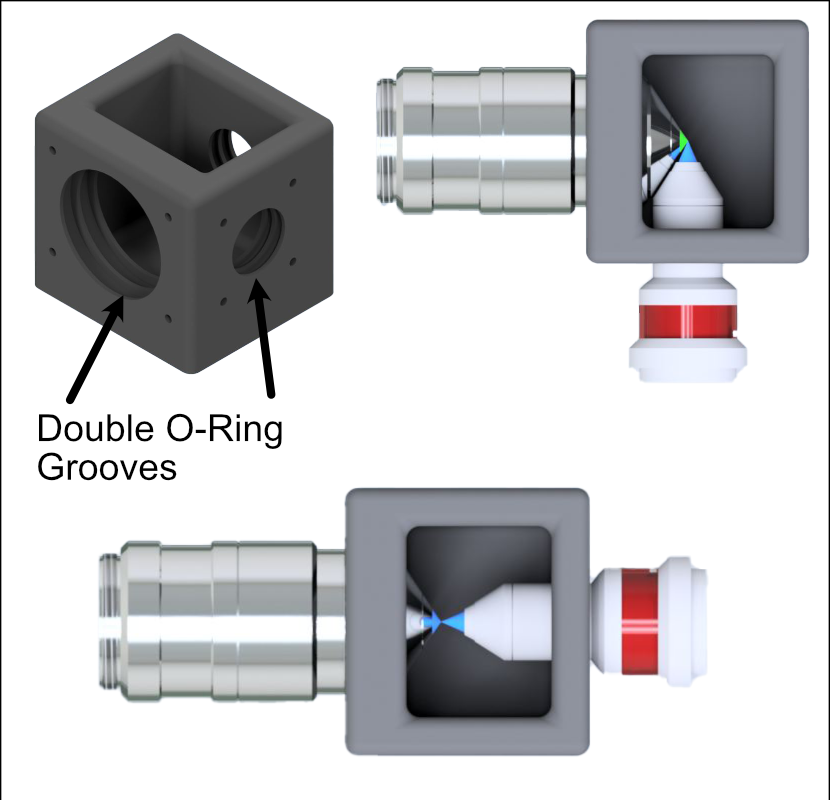
Figure 1 Two imaging configurations for the sample chamber design
Visualization of Axes Mapping
In our system we essentially have 5 different translation stages at work: the standard x,y, and z axes, an additional stage along the z axis to control the focus of the detection path (f), and and axis associated with the piezo positioned such that its normal is 60.5 degrees away from the y-axis.
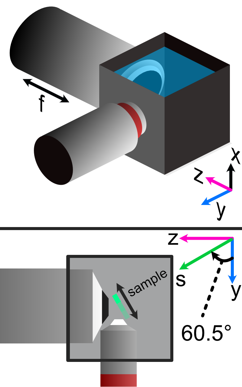
Figure 2 Layout of how the axis of the system are mapped
Minimizing Spherical Aberrations
Once the system has been assembled to the point of being able to take image stacks, the process of minimizing the effects of spherical aberrations can begin. Spherical aberrations are typically introduced into optical systems due to the surface curvature of different lens elements. This type of aberration typically presents itself visually as a sort of stretching or bending of the focus of light in the system. Certain microscope objectives, such as the Nikon 25x/1.1 NA that we employ in this setup, have a built-in collar that can be adjusted to minimize spherical aberration.
In our system, we expect the effects of spherical aberrations to be along the axis of our detection path (defined as z in our imaging scheme). In order to visualize these effects and adjust the correction collar of our objective to mitigate them, we employ a process of taking a z-stack of fluorescent beads suspended in agarose and using ImageJ to quickly process those images.
Take a z-stack within navigate of your sample
Open up the z-stack within ImageJ
Reslice the z-stack (Image -> Stacks -> Reslice)
Do a maximum intensity project of the resliced stack (Image -> Stacks -> Z-Projection)
Take note if spherical aberration is present in the projected image.
If spherical aberration is still present, make slight adjustments to the objective correction collar and repeat Steps 1-5. Each time you adjust the correction collar, you will likely need to update the focus of the microscope.
As a note, observing the camera live-feed via navigate’s “Continuous Scan” mode while adjusting the correction collar can help to get in the general vicinity of the correct placement of the correction collar. An example of how change in the correction collar affect live images are shown below for fluorescent beads. Aiming to get to get the beads near the expected light sheet position to be as in-focus as possible is a general guide for what direction to move the collar; however, true correction needs to be done with the z-projection method mentioned above.
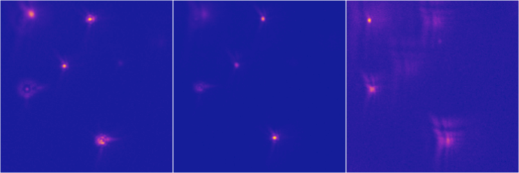
Figure 3: Effects of adjusting the correction collar when imaging fluorescent beads
As a quick example of what an image of a z-projection could look like before and after trying to correct for spherical aberration is shown below. Here, one can see in the top panel that the bead features are essentially smoothed out and fuzzy due to aberrations, while in the bottom panel with adjustments made to the correction collar the beads appear much cleaner and focused.
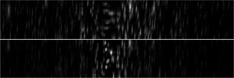
Figure 4: Before and after of adjusting in Z-projections after adjusting the correction collar
Sample Image Examples
When imaging samples, it is important to note the way in which the individual images comprising our z-stack might look as it might differ from what one might traditionally be accustomed to. In our imaging scheme, we essentially have a thin column of light spanning the vertical direction on our image. This results in each image in the z-stack being a thin snapshot of the whole sample, which can then be viewed through max intensity projections in ImageJ. To give a visual reference of what these individual images in a stack can look like for a biological sample, we provide the following images taken of a mouse embryonic fibroblast sample at a single z-position in a stack for 4 different imaging channels (gold = actin, gray = tubulin, cyan = nuclei, and magenta = Golgi apparatus).
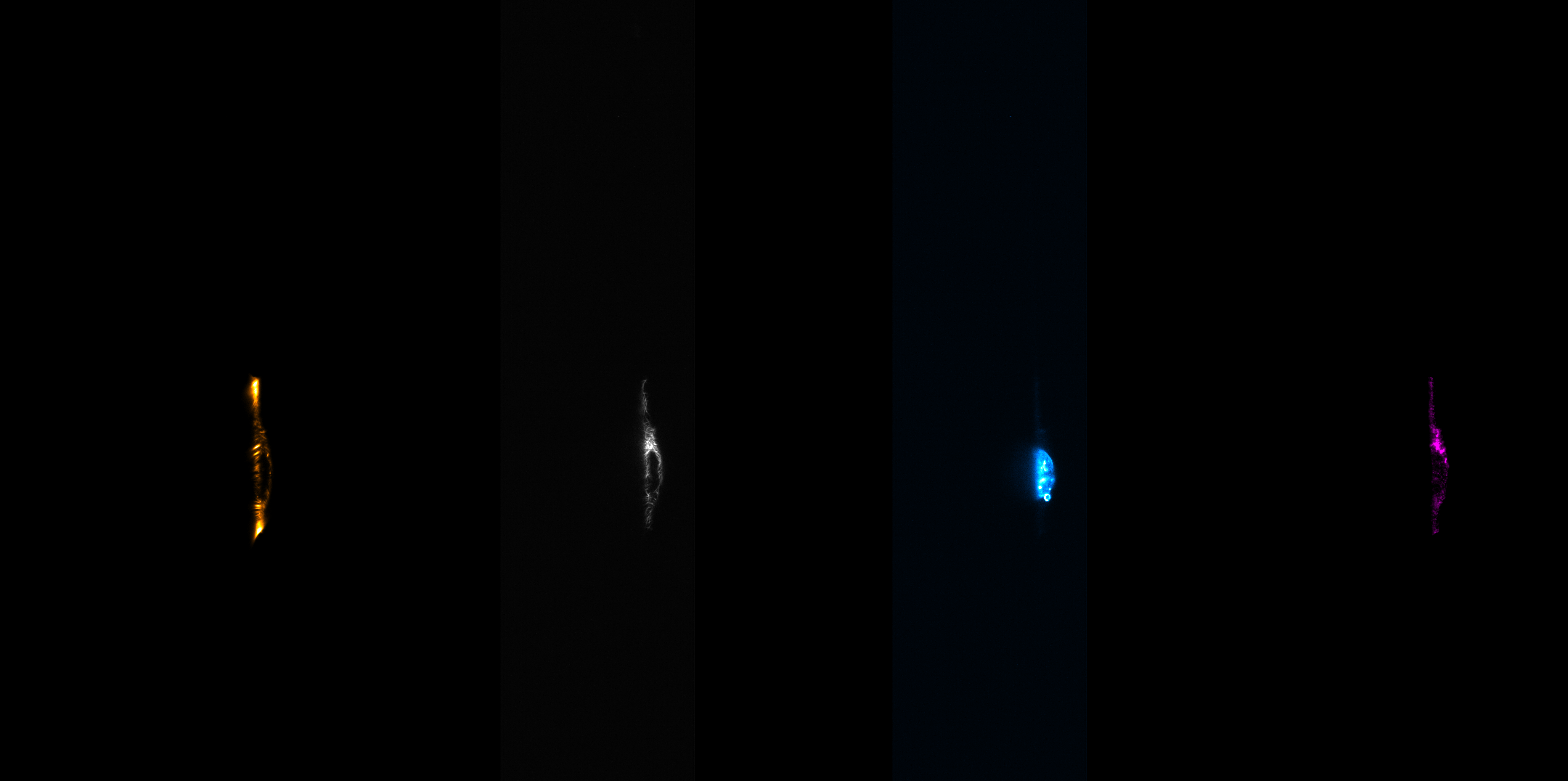
Figure 5: Example individual images for MEF cells
Image Stack Processing
Deskewing
With an image stack acquired, some post processing is still required in order to remove the effects of shearing in our images. The root of this shearing is due to the angled method in which our sample is mounted and similarly, the angled path that the sample moves as the piezo is scanned. A basic visual idea of how deskewing affects the resulting image is shown below for 100 nm fluorescent beads. Here before deskewing for the same image plane (yz), the beads appear to be stacked in a straight line but oriented along an angle, which is not the most accurate representation of our system. On the deskewed image on the right, one can see that the beads are now properly angled correspond to our piezo angle mount, and that the PSFs of the beads is now correctly aligned along the z axis.
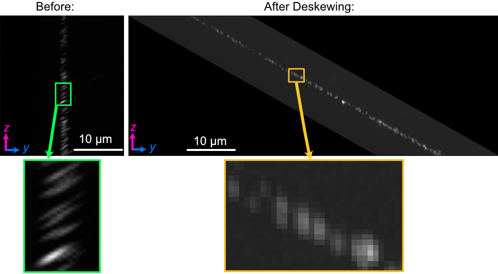
Figure 6: Difference between an image set of 100 nm bead before deskewing (left) and after (right)
To do this deskew processing, we utilize custom-built python code via Jupyter notebooks available here. The user needs to provide the correct file path to the .tif image stack collected via navigate, as well as the parameters of the imaging system like z-step size, xy pixel size, and the angle that the images should be deskewed over. In our case, our deskew angle is equivalent to 90-60.5 degrees, where 60.5 degrees corresponds to the difference between the normal of our angle mount and the y-axis. If this value is unknown, one can use different values for the deskew angle until the bead PSFs are correctly aligned along the z-axis and not angled.
Reslicing
Reslicing in ImageJ is a process that allows one to be able to reconstruct different planes of a 3D image set. In other words, it allows one to view the XY, XZ, and YZ projections of the same image set. In our system, our default viewing plane is the XY plane, and so we reslice to observe the XZ and YZ planes. The reslicing process within ImageJ is done after deskewing, and involves opening up the Reslicing panel (Image-> Stacks-> Reslice). Within this panel, one just needs to select the direction of the reslice (typically just top or left). For our system, top slicing provides us with the YZ plane view where one can observe the angled orientation of our sample setup after projection (Image-> Stacks-> Z Project). This is shown below for the same 100 nm bead samples used in the Deskewing and Rescaling portions of this page.
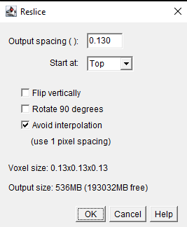
Figure 7: Reslicing Panel for top reslicing
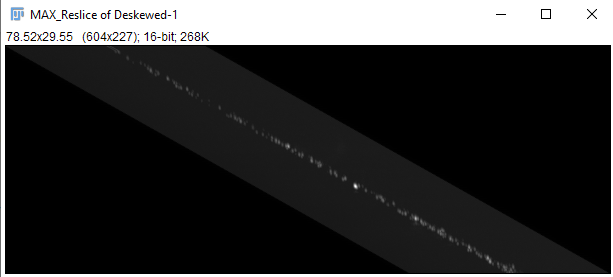
Figure 8: The YZ projection of our bead images after reslicing.
The same process can then be done to obtain the XZ plane view of our sample by reslicing left instead:
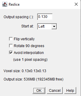
Figure 9: Reslicing Panel for left reslicing
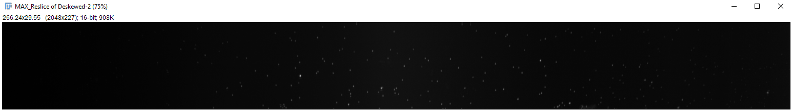
Figure 10 The XZ projection of our bead images after reslicing.
Deconvolution
Deconvolution is an iterative post-processing technique that aims to enhance the resolution of a given image. Typically, in order to properly utilize deconvolution techniques one needs not only to have an image that they want to enhance, but also have an image of the corresponding point-spread-function (PSF) of the system used to take the image. We generate this PSF through taking an image stack of an isolated 100 nm fluorescent bead. For deconvolution we utilize PetaKit5D, which is open-source and MATLAB-based image processing code base. It should be noted that deconvolution techniques, while powerful, are also highly dependent on a variety of sensitive input parameters, and finding an effective combination of these parameters can often be a difficult process.