Rendering biological data with napari#
Question: how can we show the spatial arrangement and movement of structures in a living cell clearly, without confusing a display choice with a biological measurement?
In this three-hour workshop you will load microscopy images, explore 2D and 3D views, add existing particle detections and tracks, and make a short movie. You do not need prior programming experience. Run cells from top to bottom, pause at each Try it, and change one setting at a time.
The two channels are named DNA and Mitochondria, following the source rendering notebook. The data come from Fiolka and Dean, 2026, CC BY 4.0. We use the filtered, fourfold spatially reduced teaching derivative. All 30 acquired timepoints and the original detection/track coordinates are retained. Detection and linking were performed beforehand; adding these layers does not run an analysis algorithm.
This release uses source-voxel coordinates and frame indices while physical calibration is being confirmed. Do not interpret a voxel distance as micrometres or playback fps as the acquisition rate.
1. Run your first cells#
Choose Python (napari workshop). Click the next code cell and press Shift+Enter. Lines starting with # are explanations for humans. = gives a value a name so later cells can reuse it. You can always return to a working setting.
%gui qt
from pathlib import Path
import numpy as np
import pandas as pd
import tifffile
import napari
These imports provide folder handling, arrays, tables, TIFF reading, and the viewer. %gui qt keeps the desktop viewer responsive alongside Jupyter. It belongs in a notebook, not in a .py script. Select the right kernel if an import fails.
from pathlib import Path
ROOT = next(p for p in (Path.cwd(), *Path.cwd().parents)
            if (p / "data" / "zenodo-manifest.json").is_file())
DATA = ROOT / "data" / "teaching"
print(DATA)
DATA names your extracted teaching dataset. If the next cell reports a missing file, use the download instructions and confirm that metadata.json, ch0, and ch1 are directly inside data/teaching. A browser download is equivalent to the script route.
2. Open a single image#
A volume is a pile of 2D images. Its axes here are z, y, x: depth, row, column. Each stored number is an intensity. shape tells us how many samples there are along each axis; dtype tells us how the numbers are stored.
first_volume = tifffile.imread(DATA / "ch0" / "frame_000000.tif")
print("Shape (z, y, x):", first_volume.shape)
print("Stored number type:", first_volume.dtype)
print("Memory in MiB:", first_volume.nbytes / 2**20)
Expect (30, 166, 215) and uint16 for the prepared package. This is one timepoint from one channel, approximately 2 MiB. The original volume was (118, 664, 860); reduction made it manageable while losing fine detail.
Square brackets select part of an array. The next cell selects one z plane. Python counts from zero, so the first plane is 0. A comma separates function arguments; names such as colormap= explain the setting.
z_plane = 10
viewer = napari.Viewer(ndisplay=2)
dna = viewer.add_image(first_volume[z_plane], name="DNA slice", colormap="gray",
                       contrast_limits=(0, 650))
In napari: locate the layer list on the left, the image canvas, and the selected layer’s controls. Use the mouse wheel or trackpad gesture to zoom; drag to pan. Use the reset-view button if the image leaves the window.
Try it: change z_plane to 15 and run the next cell. Predict whether the image or the display colors will change. Why would a single plane show fewer structures than the whole cell?
z_plane = 15
dna.data = first_volume[z_plane]
Checkpoint: explain what first_volume[10] selects. Answer: the eleventh z plane; it does not select timepoint 10.
3. Choose a useful display#
Contrast limits map stored intensities to screen brightness. A value above the upper limit is saturated in the display. Changing these limits does not rewrite the TIFF or alter measured values in the array.
Try the contrast controls in napari, then run the next cell to set a reproducible view.
dna.contrast_limits = (0, 650)
dna.colormap = "green"
dna.gamma = 1.0
Try it: change gamma to 0.7 and back to 1.0; compare dim structures. Change the upper contrast limit to 200, then restore 650. Describe what becomes easier to see and what information becomes harder to distinguish. Avoid comparing intensities between panels whose display settings differ without saying so.
Add the second channel from the same timepoint and z plane. additive blending lets the two colored images contribute to the combined view. Green and magenta help distinguish channels, but bright overlap alone does not prove biological interaction.
mito_volume = tifffile.imread(DATA / "ch1" / "frame_000000.tif")
dna.blending = "additive"
mito = viewer.add_image(mito_volume[z_plane], name="Mitochondria slice",
                        colormap="magenta", contrast_limits=(200, 2400),
                        blending="additive")
Try it: toggle each layer’s visibility with its eye icon. Set mito.opacity to 0.5, then back to 1.0. Explain why the colors are visualization choices, not the specimen’s natural colors. Use single-channel grayscale views when judging faint features.
4. Explore depth and time#
We will replace the two slice layers with complete time series. clear() removes displayed layers; it does not delete your files. The helper below checks the dataset and collects the timepoints. Its readable implementation is in src/napari_workshop/data.py; the optional large-data notebook walks through lazy loading.
downsample=4 means one displayed spatial sample for every four source samples along each spatial axis. The downloaded package already has this factor. It cannot recover original detail by setting this value to one. This small example loads all frames into RAM; approximately 123 MiB for both image arrays.
from napari_workshop.data import load_images, load_tables
DOWNSAMPLE = 4
images, image_scale, metadata = load_images(DATA, downsample=DOWNSAMPLE, lazy=False)
print("Channel shape (t, z, y, x):", images[0].shape)
print("Both channels, MiB:", sum(a.nbytes for a in images) / 2**20)
print("Image scale:", image_scale)
viewer.layers.clear()
dna = viewer.add_image(images[0], name="DNA", colormap="green", scale=image_scale,
                       contrast_limits=(0, 650), blending="additive")
mito = viewer.add_image(images[1], name="Mitochondria", colormap="magenta", scale=image_scale,
                        contrast_limits=(200, 2400), blending="additive")
viewer.dims.axis_labels = ("frame", "z", "y", "x")
In napari: two sliders now appear in 2D mode: frame and z. Move only z, then move only frame. Which changes location within a volume, and which changes the acquired timepoint? Timepoints run from 0 to 29.
The scale tuple says one time-index step and four source voxels per displayed spatial step. It prevents the reduced image from shrinking relative to particles stored in the original coordinate system.
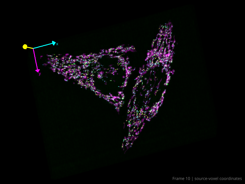
Click napari’s 2D/3D toggle, or use the next cell. 3D rendering displays a volume; it does not add another acquired dimension.
viewer.dims.ndisplay = 3
dna.rendering = "mip"
mito.rendering = "mip"
viewer.reset_view()
Try it: rotate the cell, zoom, and change the frame slider. mip selects the maximum intensity encountered along each viewing ray. Change one image layer’s rendering mode to attenuated_mip or iso using the controls, then return to mip. An isosurface is controlled by an intensity threshold; it is not automatically a segmented biological boundary.
Checkpoint: a thin bright structure may disappear in one rendering mode. Does that establish that it was absent from the measured data? Explain why not.
5. Compare a projection with a volume#
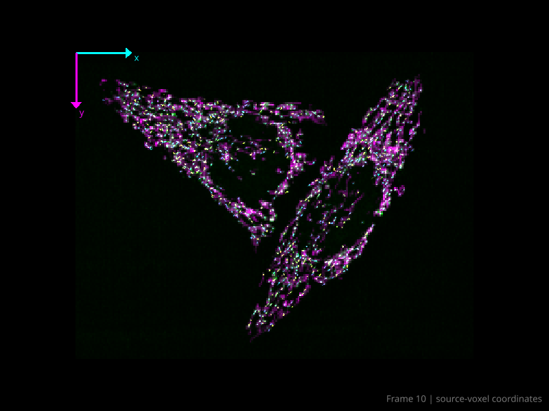
A maximum-intensity projection collapses depth: at every y,x position it retains the brightest z voxel. axis=1 means z in our t,z,y,x array. A crossing in a projection may join objects that are separated in depth.
dna_projection = images[0].max(axis=1)
mito_projection = images[1].max(axis=1)
print("Projection shape (t, y, x):", dna_projection.shape)
viewer.layers.clear()
viewer.dims.ndisplay = 2
projection_scale = (image_scale[0], image_scale[2], image_scale[3])
viewer.add_image(dna_projection, name="DNA projection", colormap="green",
                 scale=projection_scale, contrast_limits=(0, 650), blending="additive")
viewer.add_image(mito_projection, name="Mitochondria projection", colormap="magenta",
                 scale=projection_scale, contrast_limits=(200, 2400), blending="additive")
viewer.dims.axis_labels = ("frame", "y", "x")
Try it: find a feature that appears to overlap another in the projection. Remember it when you return to 3D. Break: take 10 minutes; leave your notebook and napari open.
6. Add existing particle detections#
Open the detection table. Each row is one observation with a frame number and a position. amp and int are source feature columns; do not assume either is a calibrated quantity without the detection method’s definition.
detection_table = pd.read_csv(DATA / "detections.csv")
detection_table.head()
Selecting named columns avoids mixing x,y,z order. For a projection we omit z but keep frame. We use a small helper once to validate bounds and select only the loaded frames. No particle positions are being detected here.
Image pixels were reduced fourfold, but table coordinates remain in original source voxels. The points therefore use a spatial scale of one (or the confirmed source voxel spacing); applying the image’s factor of four to them would move the particles to the wrong places.
detections, tracks = load_tables(DATA, metadata)
spacing = metadata.get("voxel_size_um") or 1
point_scale = (1, spacing, spacing, spacing)
points_2d = detections[["t", "y", "x"]].to_numpy()
particles = viewer.add_points(points_2d, name="Particles", size=4 * spacing,
                              scale=(1, spacing, spacing), face_color="cyan",
                              border_color="white", opacity=0.7)
Try it: select the Particles layer, change point size, and toggle visibility. Examine frame zero and frame ten. A larger marker is easier to see but does not mean a larger measured particle. Dense markers can obscure the image; alternate between overlay and image-only views.
Checkpoint: what do you lose when displaying only t,y,x? Answer: the particle’s depth. All detections at that frame are projected, not restricted to one z slice.
7. Add existing tracks#
A track associates observations across time. The source track CSV is headerless: its columns are track_id,t,z,y,x. The extra ID column tells napari which observations to join. This is different from a points table. The validating helper returns rows sorted by track ID and then time.
track_table = pd.DataFrame(tracks, columns=["track_id", "t", "z", "y", "x"])
track_table.head()
tracks_2d = tracks[:, [0, 1, 3, 4]]
track_layer = viewer.add_tracks(tracks_2d, name="Tracks", scale=(1, spacing, spacing),
                                tail_length=5, tail_width=2)
viewer.dims.set_current_step(0, 10)
tracks[:, [0,1,3,4]] keeps every row (:), then selects ID, frame, y, x. Tail length is a time window; here time is measured in frame-index units. It does not mean five particles. At frame zero there is no earlier history, so advance the slider before judging whether tracks are present.
Try it: change track_layer.tail_length to 15, then back to 5. Hide Particles if the display is crowded. Follow one trajectory through adjacent frames. Could a link be incorrect? Rendering a tracking result is not validation of the tracking algorithm. Choose a potential ambiguity and explain what additional evidence you would inspect.
8. Return to 3D with the same coordinates#
This cell recreates the scene explicitly so its state is known before movie export. It reuses arrays already loaded in RAM. Keep this viewer open while running the movie cells.
viewer.layers.clear()
viewer.dims.ndisplay = 3
viewer.add_image(images[0], name="DNA", scale=image_scale, colormap="green",
                 contrast_limits=(0, 650), blending="additive", rendering="mip")
viewer.add_image(images[1], name="Mitochondria", scale=image_scale, colormap="magenta",
                 contrast_limits=(200, 2400), blending="additive", rendering="mip")
viewer.add_points(detections[["t", "z", "y", "x"]].to_numpy(), name="Particles",
                  scale=point_scale, size=4 * spacing, face_color="cyan", opacity=0.7)
viewer.add_tracks(tracks, name="Tracks", scale=point_scale, tail_length=5, tail_width=2)
viewer.layers["Particles"].visible = False
viewer.dims.axis_labels = ("frame", "z", "y", "x")
viewer.dims.set_current_step(0, 10)
viewer.reset_view()
9. Save a screenshot#
Choose a view and contrast settings. We create a fresh output folder for this run so earlier exports are preserved. A screenshot stores the rendered view, not the full-dimensional microscopy data. Your original TIFFs and table files remain unchanged.
from datetime import datetime
OUTPUT = ROOT / "outputs" / datetime.now().strftime("lesson-%Y%m%d-%H%M%S-%f")
OUTPUT.mkdir(parents=True)
viewer.screenshot(path=OUTPUT / "my-view.png", canvas_only=True, size=(480, 640))
print("Saved in:", OUTPUT)
Open my-view.png from the Jupyter file browser or Finder/File Explorer. Check that the crop, colors, and tracks match your intent. The size argument is height, width, so this image is 640 pixels wide and 480 high. We are not adding a physical scale bar until calibration is confirmed.
10. Make a short movie#
There are two distinct kinds of change: the camera moves around a fixed acquired volume, or the acquired timepoint changes with a fixed camera. Start with camera movement.
In napari, open Plugins → napari-animation: wizard. Capture a view, rotate gently, capture another, and preview. The plugin interpolates viewing settings between those keyframes; it does not generate new biological observations. If you cannot find the plugin, the next cell shows the equivalent short script.
from napari_animation import Animation
animation = Animation(viewer)
viewer.dims.set_current_step(0, 10)
viewer.camera.angles = (0, 0, 90)
animation.capture_keyframe()
viewer.camera.angles = (20, 25, 110)
animation.capture_keyframe(steps=30)
capture_keyframe() remembers the current viewer state. steps=30 requests a short transition to the next state. Both states use the same acquired frame. Export below; wait for the cell to finish before manipulating napari. A blank preview or failed encoding is addressed in troubleshooting.
animation.animate(str(OUTPUT / "camera-movie.mp4"), fps=10, canvas_only=True)
print(OUTPUT / "camera-movie.mp4")
Now create a movie of acquired timepoints with a fixed camera. This readable loop writes one rendered image per source timepoint. The helper in src/napari_workshop/render.py adds automatic verification for the standalone example, but the essential actions are shown here.
with opens the encoder and closes it when finished. for repeats the indented lines for every frame. Updating the frame slider changes the volume. processEvents() lets the viewer draw that change before capturing it. A screenshot includes an alpha/transparency channel; :,:,:3 retains just red, green, and blue for the movie. Frames are written one at a time, avoiding a second large list in RAM.
import imageio.v2 as imageio
from qtpy.QtWidgets import QApplication
fps = 5
viewer.text_overlay.visible = True
with imageio.get_writer(OUTPUT / "time-series.mp4", fps=fps, codec="libx264",
                         pixelformat="yuv420p", macro_block_size=16) as writer:
    for t in range(images[0].shape[0]):
        viewer.dims.set_current_step(0, t)
        viewer.text_overlay.text = f"Frame {t}"
        QApplication.processEvents()
        rgb = viewer.screenshot(canvas_only=True, size=(480, 640))[:, :, :3]
        writer.append_data(rgb)
At 5 playback frames per second, 30 acquired frames make a 6-second movie. This does not tell us how many seconds elapsed in the experiment. Verify the exported file rather than assuming it worked because no error appeared.
with imageio.get_reader(OUTPUT / "time-series.mp4") as reader:
    print("Movie frames:", reader.count_frames())
    print("Playback fps:", reader.get_meta_data()["fps"])
    print("Movie dimensions:", reader.get_meta_data()["size"])
print("Open the movie in your usual video player:", OUTPUT)
Check: 30 frames, 5 fps, and (640,480) dimensions. Watch the beginning and end. Are tracks visible? Does the frame label change? Did the camera stay fixed? Saving a file is not the same as verifying its contents.
11. Your independent challenge#
Create a view that answers one biological question. Choose the channels, contrast, dimensional view, and whether to show particles or tracks. Save a screenshot or short movie and explain three choices to a neighbor.
Discuss: (1) what depth information your view preserves, (2) how its display settings affect interpretation, (3) why displayed tracks can still contain errors, and (4) what you would need to report a speed in micrometres per second.
Save your notebook with Ctrl+S on Windows or Command+S on Mac. Kernel restart clears variables; rerun from the top to reconstruct them. The quick reference helps you repeat the workflow. Continue with the optional animation or large-data notebooks when time permits.
Finish: close the napari viewer using the next cell when you are ready. Keep your original data and your exported files.
viewer.close()