Optional: downsampling and loading data only when needed#
Question: how can we explore an image sequence that does not fit comfortably in RAM?
This notebook first uses the small dataset so you can learn safely. The original dataset is about 8.1 GB on disk. To use original images, run the documented source download before class: uv run scripts/download_data.py --dataset source --timepoints 5 in a terminal opened in the workshop folder. That still transfers about 1.35 GB. --dry-run reports sizes without downloading. Downloading only five timepoints retains a short contiguous sequence so tracks and time indices stay meaningful.
A smaller download, spatial downsampling, and lazy loading solve different problems. Lazy loading from your local disk does not eliminate the download. A compressed TIFF may need to be decoded as a complete volume even when you only want one slice.
Inspect what downsampling changes#
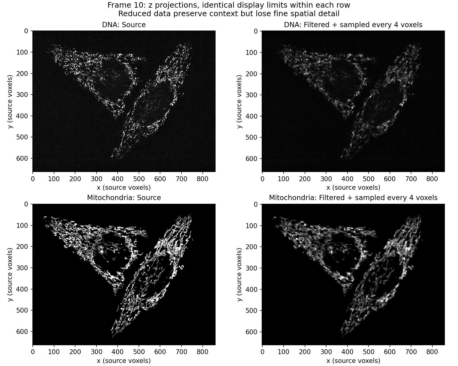
These are real maximum-intensity projections with the same contrast limits within each channel. Factor-4 spatial downsampling preserves broad structure but removes fine detail. It is intended for this visualization lesson, not a replacement for the source data in quantitative analysis. The filtering and sampling preserve the original voxel centers at indices 0, 4, 8, …; the last displayed voxel edge can differ from the source edge by less than half a coarse voxel. We do not stretch the image to force the outer edges to match, because that would move the sampled centers relative to the points.
%gui qt
from pathlib import Path
ROOT = next(p for p in (Path.cwd(), *Path.cwd().parents)
            if (p / "data" / "zenodo-manifest.json").is_file())
DATA = ROOT / "data" / "teaching"
print(DATA)
Choose the dataset and total spatial factor. The prepared teaching package is already reduced by four: it supports factors four or eight, not one or two. For original source data, factors one, two, four, and eight are available. Keep time unchanged. Begin with the working default.
DATASET = "teaching"  # change to "source" only after downloading original files
DOWNSAMPLE = 4         # total factor relative to the original spatial grid
LAZY = True
DATA = ROOT / "data" / DATASET
Dask can represent an array as a set of instructions to load pieces later. We set a single local worker so concurrent reads cannot unexpectedly fill memory. The helper validates TIFF headers and stacks one delayed read per timepoint/channel. It reads no image pixels while constructing the lazy array.
import dask
from napari_workshop.data import load_images, load_tables
dask.config.set(scheduler="single-threaded")
images, image_scale, metadata = load_images(DATA, downsample=DOWNSAMPLE, lazy=LAZY)
print("Array type:", type(images[0]).__name__)
print("Shape:", images[0].shape)
print("Logical size of both arrays, MiB:", sum(a.nbytes for a in images) / 2**20)
print("Chunks:", images[0].chunks if LAZY else "eager NumPy array")
nbytes here describes how much space the entire resulting array would occupy if materialized. It is not a measurement of current RAM use. Calling compute() on the entire array would load all frames. Calling it on a single selected volume loads just that volume’s task.
Here is the essential pattern behind the helper. It constructs a delayed read of one real TIFF. The image is filtered in float32 before subsampling at original-grid positions; rounded uint16 values are returned. Filtering reduces aliasing, but the result has less spatial detail.
from dask import delayed
import dask.array as da
from napari_workshop.data import image_path, read_volume
path = image_path(DATA, channel=0, time=0)
relative_factor = DOWNSAMPLE // metadata["spatial_factor"]
task = delayed(read_volume)(path, relative_factor)
one_volume = da.from_delayed(task, shape=images[0].shape[1:], dtype="uint16")
print(one_volume)
delayed records a call without running it. from_delayed tells Dask the resulting array’s shape and storage type. The next cell asks for that one volume and measures its loading/reduction time. A second visit may behave differently due to operating-system caching; do not call this a formal benchmark.
from time import perf_counter
start = perf_counter()
first = one_volume.compute(scheduler="single-threaded")
print("Seconds for this read:", round(perf_counter() - start, 3))
print("Loaded volume MiB:", first.nbytes / 2**20)
The full viewer accepts the lazy arrays. Moving to another acquired timepoint requests another stack. A movie still has to read every timepoint it renders. GPU rendering works on the displayed volume; lazy loading does not automatically make that volume smaller.
import napari
viewer = napari.Viewer(ndisplay=3)
viewer.add_image(images[0], name="DNA", scale=image_scale, colormap="green",
                 contrast_limits=(0, 650), blending="additive")
viewer.add_image(images[1], name="Mitochondria", scale=image_scale, colormap="magenta",
                 contrast_limits=(200, 2400), blending="additive")
detections, tracks = load_tables(DATA, metadata)
spacing = metadata.get("voxel_size_um") or 1
viewer.add_tracks(tracks, name="Tracks", scale=(1, spacing, spacing, spacing),
                   tail_length=5, tail_width=2)
viewer.dims.axis_labels = ("frame", "z", "y", "x")
Try it: close this viewer, change the factor from four to eight, then rerun from the settings cell. Predict the size change: halving each of three spatial dimensions reduces voxel count roughly eightfold. Compare visible fine detail and whether tracks still align. Do not move the tracks to compensate by eye; the coordinate mapping must be correct.
Images use the total spatial factor in their scale. Particle and track positions remain in source coordinates and use only the source voxel spacing. Multiplying their positions by the factor again would be an error.
Memory reminders: keep one viewer open; avoid whole-series compute() or persist(); a hidden layer can still hold data in RAM; restart the kernel if you need to release all notebook references. Using LAZY=False is reasonable for the small prepared data, but first calculate the full logical size.
The original files and excluded timepoints are preserved. Loading the first five frames filters the display tables to those frames; it does not claim that a truncated track began or ended biologically at the subset boundary.
viewer.close()